


This is part five of a six-part series exploring spending optimization in Major League Baseball. Each article will dive deep into different ways that teams spend their dollars to produce the best value. You can find part one (and the rest of the series) here.
In general, good organizations need to be willing to change based on a situation, not anchoring to given strategies because they worked in the past. This flexibility has oftentimes been the key to survival, and baseball teams are no exception to this. As the environment changes (from increased levels of overall runs, different baseballs, new technology, etc.), these teams need to be willing to alter their strategy based on their present situation. A major aspect of this flexibility that goes hand-in-hand with spending optimization is the willingness to vary investment size, based on the given environment.
What is the effect, if any, of investing dollars in certain times versus others? And to that extent, when would these possible times be? Scaling investments for given times has been a popular tool for many major Financial players; its application in the baseball world is now called into question. It is likely that such an effect exists, although the degree of said effect could be abysmal. The following research will attempt to break down this question from every angle to truly uncover the best way for a team to optimize its portfolio.
Using Spotrac data, 240 teams’ seasons, win percentages, run differentials, and spending habits dating from 2013-2021 (excluding 2020) were used to conclude the matter of scaling investments. The sample includes cash spending, with adjustments for the average amount spent per year.
An Introduction to Scaling Investment
As teams often don’t get an extreme influx of cash from their owners or outside media deals, it should be of no surprise to the reader that a given team’s cash spending does not vary much from year to year. The median year-over-year change was 11.4%. The graph experienced a right-skewed distribution, with the majority of teams’ seasons failing to change more than 8% in adjusted spending (accounting for 30% of everyone). Drastic change is often looked at as unnatural, making such big changes a bit more uncommon in the grand scheme of things. Occasionally though, you run into a few teams that were willing to change it all.
During the 2014 off-season, the Houston Astros decided that they were ready to compete. Their adjusted cash spending went from 0.45 in 2014 to 0.70 in 2015 – a 58% increase in adjusted dollars spent. Of course, while this spending does appear dramatic, it was the result of years of planning after Jim Crane purchased the team in late 2011 and brought in new management to more efficiently run the club. Between 2019 and 2021, the San Diego Padres adjusted their spending drastically, increasing their adjusted investment size by 57%. This could also likely be owed to the change in ownership, with Peter Seidler taking a dedicated stance after assuming control of the team in late 2020. The two largest year-over-year changes that completely redefined their stance on spending were probabilistically due to new ownership. Such a dramatic shakeup in spending likely requires that large of a move, as most owners are generally not going to suddenly increase their player expenses by such a margin.
Both teams mentioned above acted similarly regarding their changes in spending but yielded completely different results. The Astros were able to improve their win percentage by 21.3% (to .530), while the Padres only managed to increase theirs by 13.0% (to .488) in the following season. These results chosen may seem small and selective, but this type of relationship was experienced all across the sample – shown below is the correlation between the change in Win Percentage and the percentage change in adjusted cash spending, year-over-year.
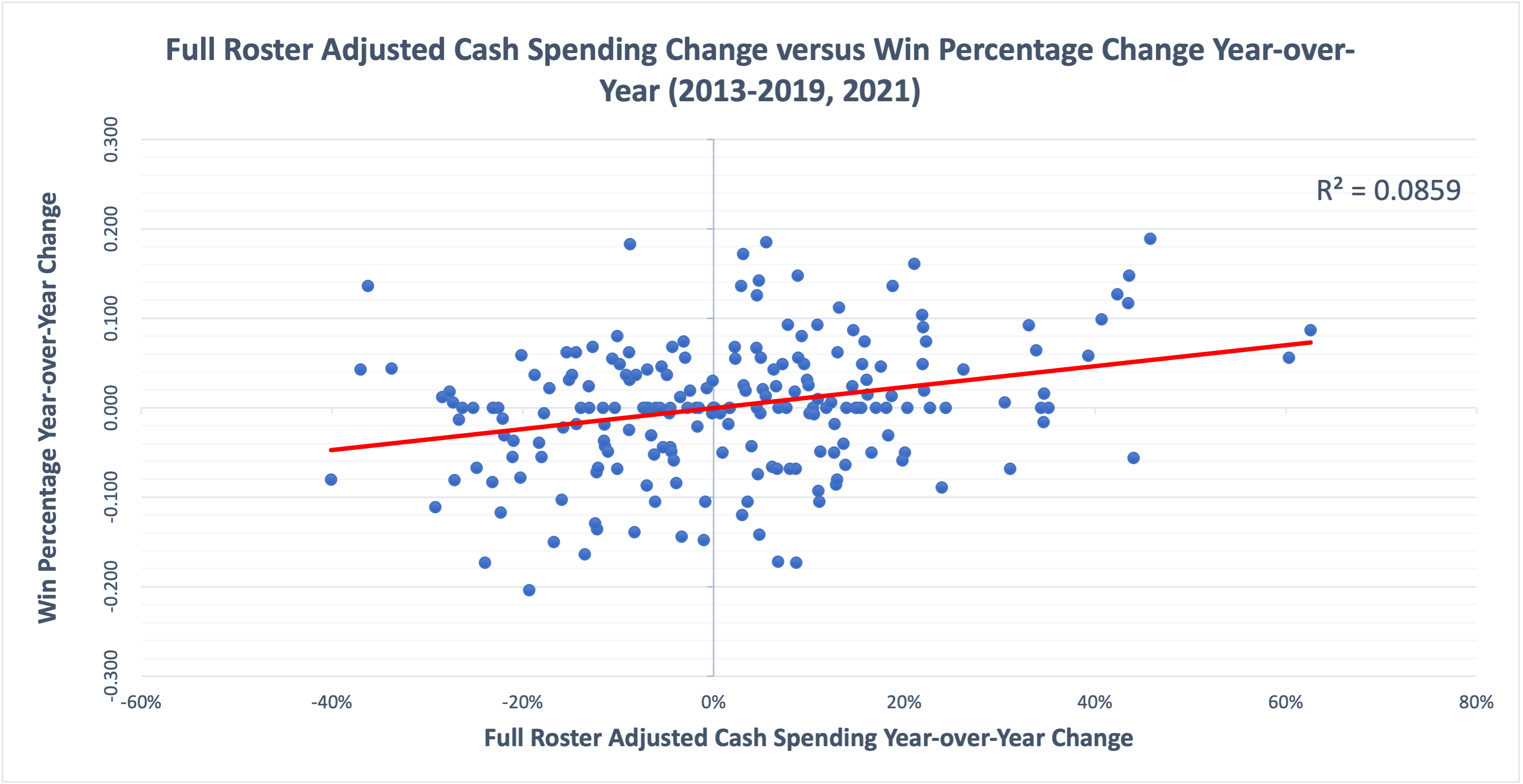
As revealed by the r-squared score, about 8.6% of the year-over-year change in win percentage could be owed to the year-over-year percentage change in adjusted cash spent. While not overly significant, this does show that teams that improve their spending from the prior year generally do better, going hand-in-hand with Part I’s conclusion that teams that spend more generally do better than those that don’t. However, it is worth noting this relationship is not as strong as the regular adjusted cash versus winning percentage mentioned in Part I, which implies that additional adjusted cash in itself has a clearer relationship with a given team’s additional percentage improvement in spending. This makes sense, as changes for cash in terms of percent can equal and mean two different monetary amounts. In terms of maximizing return, while focusing on individual improvement is important, a team is better off focusing on just trying to up the amount of cash they are spending.
There is an array of variables that were not considered in the aggregate result, which also further proves that the analysis of the different changes in spending is not yet complete. The issue needs to be looked at from all angles – not just a singular regression. The overall result somewhat oversimplifies the natural complexity of such an issue, as it generalizes the nature of a team’s actions on spending into a singular point. While the broad singular point may prove that most teams may not benefit from a change, a small subset in the optimal positions could gain. These subsets, if existent, will try to be identified through the consideration of numerous team types and other external baseball factors.
Scaling Investment Based on Different Tiers of Spending
It is generally known across all types of spending that one dollar does not equal another, with each additional dollar spent usually adding less value than the one beforehand. This is commonly referred to as diminishing marginal utility – a concept that can be heavily related to spending optimization in general. Under this specific application, in theory, an additional percentage increase in adjusted cash spending would have less of an effect on a team that already spends a good amount compared to a team that does not. Within that, there are a few facets worth tackling.
For one, does this concept apply to MLB cash spending? Are percentage changes in dollars less effective for high or low payroll teams, or do the correlations justify a spread-out effect among all teams somewhat equally? Answering these questions will reveal the intrinsic qualities of the spending dollar, which sets up the second facet. Knowing these qualities, how should teams adjust or let be their cash investments? What extent of change or non-change is needed? To find a plausible answer to this, each level of spending needed to be fairly split. This was done with a quartile system, with each quarter of the cash spending scores being divided. From there, each group had an r-squared score measuring the correlation between the cash spending change. The higher the score, the more plausible it is to say that increased cash spending matters more for a particular group. The results for the four groups are charted:
To avoid confusion, these numbers were generated using the starting win percentage, with the level of change reflected in the next year. Hence, the sample was only 210 year-over-year team season changes (53 in Q1 and Q4, 52 in Q2 and Q3). The results should be weighed with such a sample size in mind.
Each quarter was below a .10 r-squared score, except for Q1, which almost yielded double that with the shown 0.175. The second was Q2, possibly suggesting that being sub-.500 sets up a decent path to improve with cash. Q4 was admittedly close to Q2 in correlation though, somewhat negating that. Q3 demonstrated complete independence, as the score was <0.001. The difference between the two latter quarters is interesting, as such a different relationship between those two levels of spending to wins would not be expected whatsoever. Such a problem falls within the margin of variance with the given sample size, hence, it is not something that needs to be overanalyzed. Besides that mixup, the actual results somewhat fall in line with the rules of diminishing marginal utility.
It was estimated that about 18% of the increased percentage in win percentage could be owed to the matter of an increased percentage in cash spending when a team spent less than 75.9% of their average opponent. With this in mind, teams with spending levels similar to or below that number would likely get a larger payoff from each dollar that they spent. Elevating investment at that time would be highly recommended, as the payoff is much greater than any other quartile. A degree of elevated investment could also be justified for some degree of the second quartile, although this should be thought of as a sliding scale. The closer a team gets to reaching the median, the less strongly advised investment would be recommended. Despite the minute but existent causation factor in Q4, anything above the median does not particularly warrant any action besides keeping up with the current rate of spending as the league has done. The relationship is frankly not strong enough and does not fall within the hypothesis of diminishing marginal returns.
On that same note, such a decrease in investment would likely have a similar effect as the increase. Teams that do not have lots of money stand to lose the biggest portion of their winning percentage if they elect to spend less cash, on average. There of course may be exceptions, as some teams do defy the seemingly flawed odds every day. But for the majority of the pack, it makes sense to go big when spending small and go smaller when spending big.
Adjusting To How Teams React in Spending to Winning
As discussed prior, it became clear that trying to beef up spending percentages when payroll was already large proved to not be very effective – only teams with lower payrolls saw much improvement in their squad. We now know this as the reality. But how did teams actually react? Teams are not perfect – especially when it comes to spending. Hence, perhaps a look into their habits and the context of reality offers a way to potentially devise optimized strategies. Within the sample, for every percentage change in Winning Percentage, the median cash score percentage changed by about 1.09. In other words, team’s spending habits changed by about 109% of their prior change in Win Percentage. Cash Spending by teams can be considered elastic relative to their win percentage change last year.
It is worth noting that there are two types of elastic change that a given team could have – positive elastic change or negative elastic change. In positive elastic change, a team is willing to spend much more given their prior success. In negative elastic change, a team is willing to spend much less as they can, in theory, afford to not win as much. There were more positive elastic seasons than negative (64 versus 33), suggesting that most teams wanted to try to win more after improving previously. The following teams demonstrated this trait over the sample:
And here are the teams with Negative Elastic Seasons:
The purpose of this section was to provide solid circumstances for how teams generally react to their prior change in win percentage in terms of cash change. From this, it is safe to say teams tend to make a bigger change in their cash spending than their prior win percentage change. In a review of the relationship, prior win percentage change had a 0.086 R-Squared Score when compared to cash change. This is derived from the correlation coefficient, which was about 0.29 in this instance. So while a causation and some form of relationship may exist, it is not overly strong. In terms of strategy, these charts at least offer some info as to how teams have reacted to their changes – whether that is predictive of future behavior is honestly unknown. Common business logic states that managers generally use their prior improvement as a benchmark, and these results reveal how they reacted to the given benchmarks. In utilizing this correctly, the key would be to identify the structure and responsibility system of a given organization. By identifying teams with a number of positive / negative elastic seasons, as well as some information regarding how opposing ownership reacts to given variations, a team could more accurately gauge the possibility of spending increasing or decreasing from their opponents. The numbers, in this case, would be more accurately used as a justification of a given information-based hypothesis or a pique of interest for further investigation – alone, it’s value is likely minimal.
If a given team is able to use both of these facets together successfully, they would likely have a significant edge over their opponents in allocating payroll. Scaling based on the market is crucial in ensuring that the most value is bought for the cheapest price. And given that managers are inherent creatures of habit in responding to changes (say, an improved Win Percentage bump), a team can adjust to the predictability accordingly and become more suited to stay above competitors.
Scaling Investment Based on Rates of Inflation
Throughout this piece, adjusting dollars has been key in figuring out the true rates of change for a given team. But what about when the environment itself changes? In navigating the facets of spending, there is possibly an exploitable advantage within the rate at which dollars inflate from year to year and how the competition responds. Before going any further, below is the Total Cash Payroll Inflation Rates by Year:
Spending during this period began growing at a rapid pace and slowly started to experience a state of disinflation, and eventually deflation after the shortened 2020 season. Of the team seasons in the sample, roughly 46.7% beat the average inflation rate. In examining the teams themselves, the following three teams had the most seasons in the sample where their increased spending outpaced the average MLB Spending Inflation:
While useful, to truly perform a thoughtful analysis of this section, the overall strategy needs to be discussed to cover the impact of inflation rates on given types of teams.
In beginning with the overall strategy, reviewing the different ways that different teams are affected by inflation is crucial. To do so, three periods of inflation will be established – extreme inflation, regular inflation, and deflation. Extreme inflation will be defined as any inflation rate above 10% (it’s not hyperinflation by definition, but it is high!), inflation will be 0-10%, and deflation is obviously any amount below 0. By examining these periods, it should become clear whether certain types of teams react to an influx of cash into the market.
The extreme inflation years will be the first part examined – this includes the 2014 and 2015 seasons, which saw an 11.35% and 10.38% increase, respectively, in spending. During this period, it appears that the teams that had higher payrolls typically increased their cash spending by less (relative to their starting payroll) than lower payroll teams. The correlation coefficient for the regression was a -0.35 (P-Value <0.01), suggesting that as a general concept, lower-payroll teams were increasing by more of their relative payroll It also suggests that a new wave of lower payroll team’s spending, not higher payroll teams, was the main reason behind this extreme inflation. The vast majority of teams that beat the average inflation rate had payrolls below the average for that given year. Of course, context is everything – higher payroll teams struggle much more to increase their relative payroll due to the main fact that they have to spend more to do so in comparison to Smaller Market teams. Still, this proves that the rich (teams) did not get richer during this period of rapid contract increases.
For the regular inflation years, or 2016, 2017, and 2019, the relationship was on a similar track, but slightly less than the extreme inflation rate. Carrying a -0.26 (P-Value <0.05) correlation coefficient now, as payroll increased, the relative increase to payroll decreased. In determining the normal relationship between these two factors, this range of inflation would be the most likely to reveal a benchmark to compare other inflationary periods. Spending is closer to evening out in this sub-sample, and larger payroll teams take up a higher percentage of increases above average than they did prior. It is likely that this is a return to the market normal.
During the deflationary years of 2021 (from 2019) and 2018, it appears as if the effect of how much cash a given roster has almost has no effect on the amount a given team chooses to increase by their relative spending. With a correlation of -0.07 (not significant) and a visible figure with no clear relation, deflationary periods must act as a time when big spenders can healthily maintain their spending while small spenders need to contract. Teams with above-average roster cash now make the majority for those who increased their cash spending.
In theorizing as to why these given inflation reactions are the case, the most likely answer relies on external factors. Within the given time of extreme inflation, this was the beginning years of the new CBA (2012-2016) which established massive revenue-sharing for teams in lower markets. Lower-market teams were hit with an influx of cash, and their consequential spending must’ve outpaced the prior rate at which large market teams were spending cash, hence the above-average inflation rate. Once the teams began to revert back to their normal spending, these rates obviously cooled, and then began to overcorrect. Once COVID-19 hit and teams had to rely on their discretionary funds to reach payroll, it appears that the bigger teams maintained their status of normalcy and the smaller market teams started to cut down any possible fat. With context, it somewhat makes sense as to why the spending adjusted during those periods.
While the sample does indicate that high-inflation times were good for lower-payroll teams and deflationary times were not, this could possibly be more indicative of this particular sample than the actual reality. In theory, large payroll teams suddenly seeing a huge boost in their media deals could see that portion increase their margin of spending by a lot, causing massive inflation. So while inflation does likely have an impact on how teams should spend, how a given team should respond depends on where that inflation is actually coming from. By knowing this, a team should be able to navigate in a more orderly fashion.
Conclusion
For choosing when to spend and when to not, the answer is not very straightforward. Different scenarios require different actions and different levels of commitment. With the right context though, certain frameworks can be applied that should make it somewhat easier to make those difficult decisions. The point of those very structures is not to say a given time or amount is absolutely right or wrong, but whether it generally can be justified. In this part discussing spending optimization theory, changing a given team’s way of spending was looked at through the amount they had already spent, the reactions of other teams, and the inflation rates of spending. Through these avenues, the reader should hopefully be more informed about the strategy behind finding the most opportune times to spend.
